Here are basic examples. First, load the libraries used in this demo and create sample data.
library(quartabs)library(tibble)library(dplyr)library(purrr)library(tidyr)library(plotly)library(htmltools)library(knitr)library(gt)library(DT)library(tinytable)library(reactable)library(flextable)# sample datadf1 <-tibble(# id: intentionally created in descending order for the examples shown laterid =paste0("id", 6:1),group1 =c(rep("A", 3), rep("B", 3)),group2 =rep(c("X", "Y", "Z"), 2),var1 =1:6,var2 =list(1, 2, 3, 4, 5, 6),var3 =factor(letters[1:6]))df1
# A tibble: 6 × 6
  id    group1 group2  var1 var2      var3
  <chr> <chr>  <chr>  <int> <list>    <fct>
1 id6   A      X          1 <dbl [1]> a
2 id5   A      Y          2 <dbl [1]> b
3 id4   A      Z          3 <dbl [1]> c
4 id3   B      X          4 <dbl [1]> d
5 id2   B      Y          5 <dbl [1]> e
6 id1   B      Z          6 <dbl [1]> f
tabset_vars, output_vars
The tabset_vars argument specifies columns to display as tab labels. The output_vars argument specifies the columns to display in the tab.
Don’t forget!
Make sure to set the chunk option to results: asis.
Default chunk options can be changed if necessary.
cat() is used internally for non-list columns to avoid unnecessary prefixes such as “[1]” in the output. On the other hand, print() is used for list columns.
For example, var1 displays “1”, while var2 of type list displays “[1] 1”.
Factor, Date and POSIXt displays
In render_tabset(), cat() is used to output for columns that are not list types. However, if cat() is used, factor, Date, POSIXt are output as an integer. So, if these are included in tabset_vars or output_vars, it is converted internally to string (after sorting by tabset_vars).
Here are some simple examples. First, define test objects.
Oops, the entire tabset is now a third of the width. We want the content within to be displayed side by side without changing the width of the tabset. This is where the layout argument comes in handy.
In narrower displays, such as on smartphones, the layout may not appear to work.
The layout argument is intended for very simple use cases, so complex layouts may not work.
heading_levels
Use the heading_levels argument if you want the heading to be displayed as normal headings instead of tabsets. heading_levels and tabset_vars correspond in order. Each tabset_vars is expressed as the heading of specified in heading_levels. If the element of heading_levels is NA, then the element of its tabset_vars is represented as tabset.
Example 1
For example, group1 should be tabset and group2 should be h4 heading.
As of 2025-03-05, the latest version of Quarto is 1.6, but the Bootstrap version used appears to be Bootstrap 5.2.2, which was introduced with Quarto 1.4.
Several tab customisations are available in Bootstrap 5.2. One of these is pills.
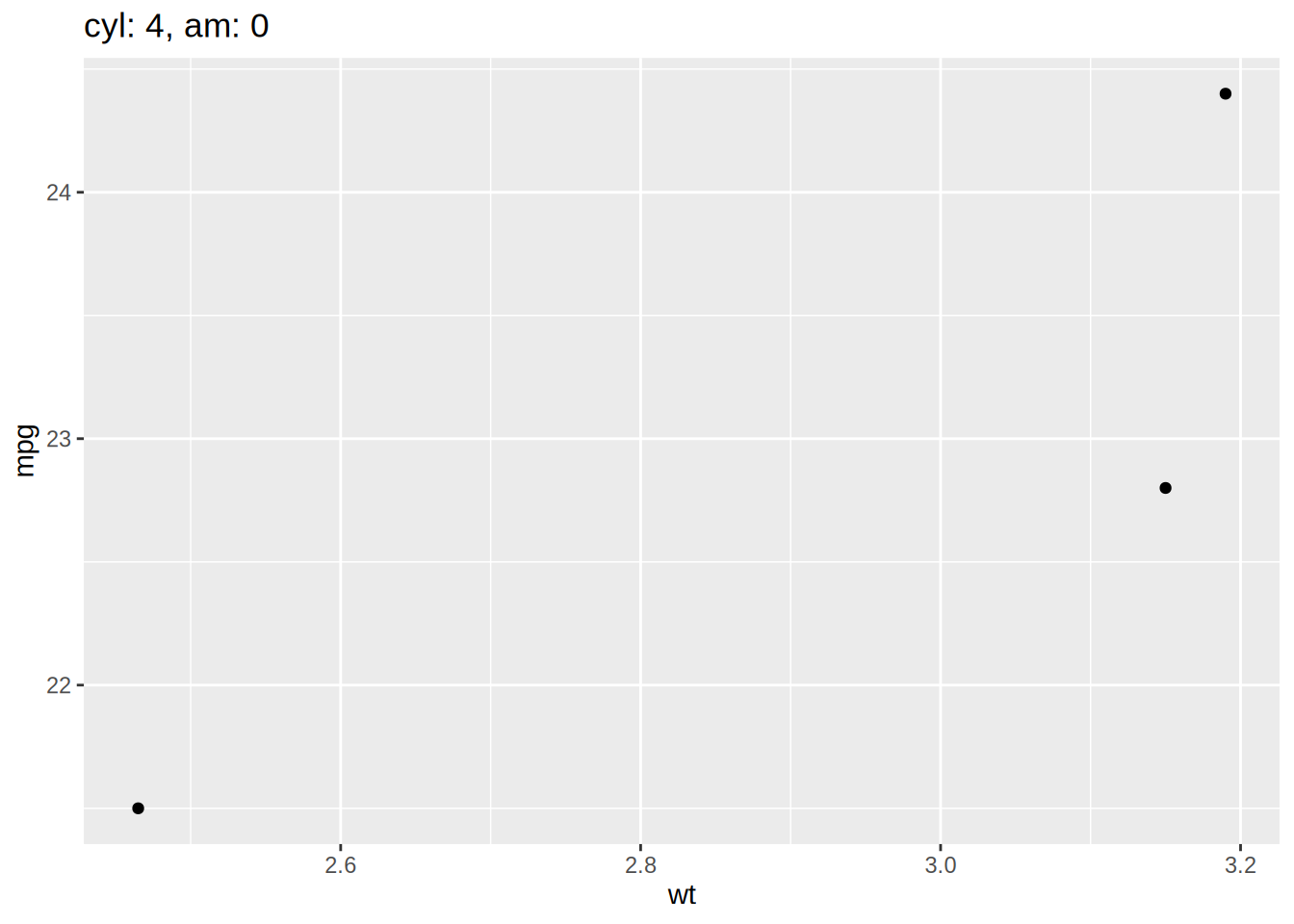
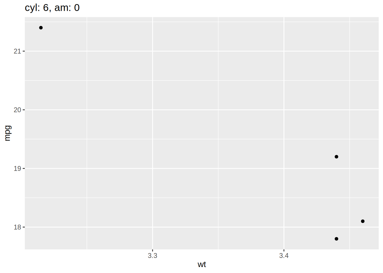
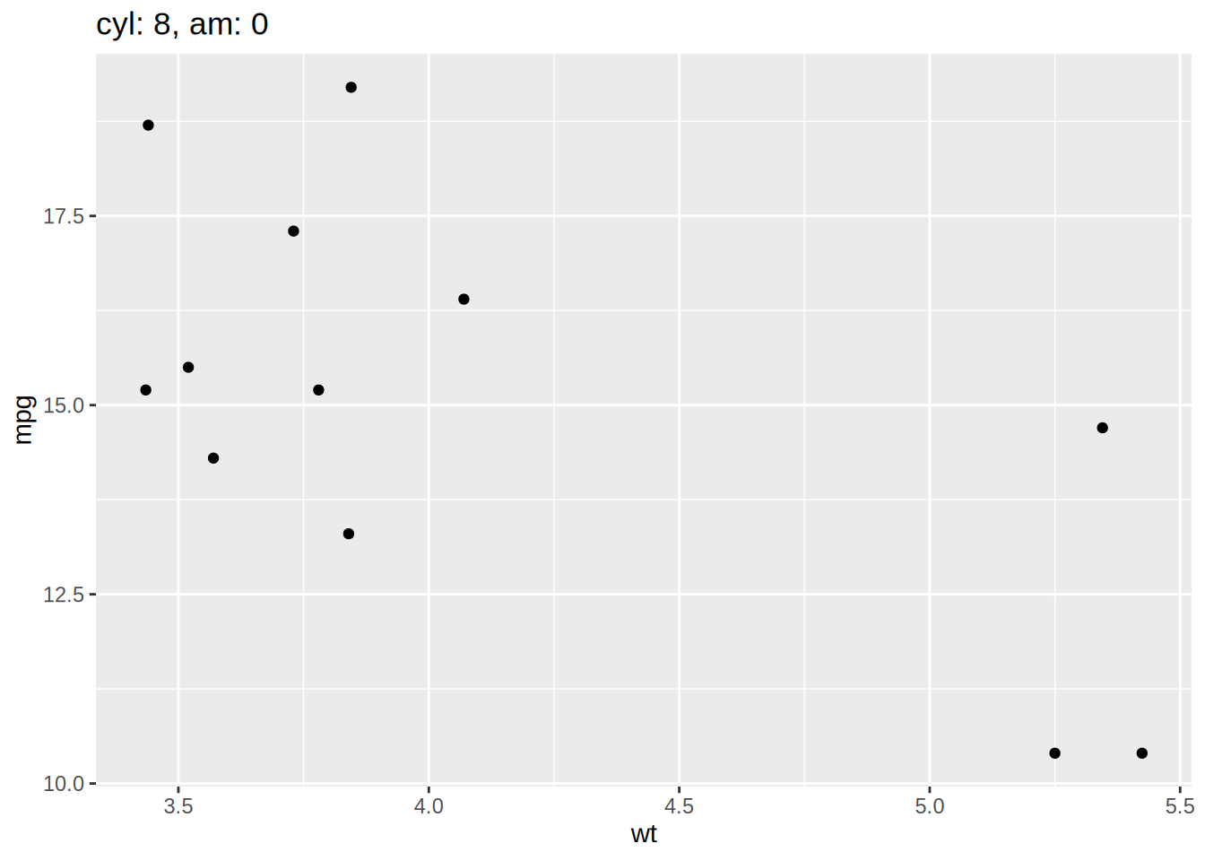
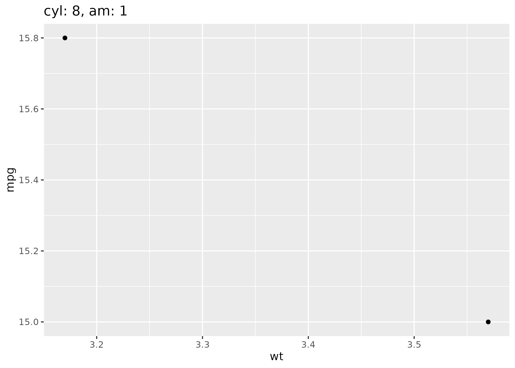
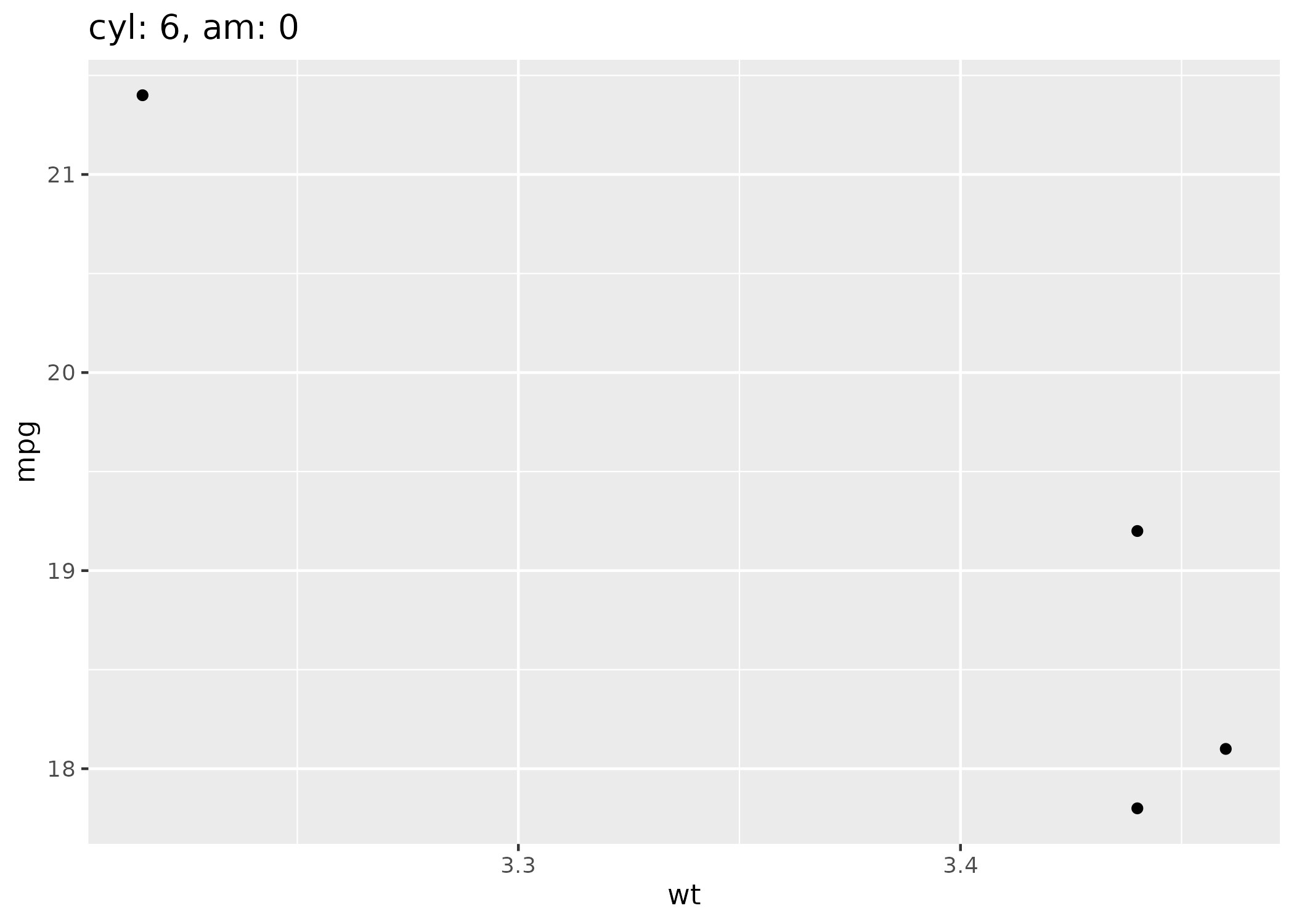
This section shows more practical examples. Use the mtcars dataset, grouped by cyl and am, to create figures and tables showing the relationship between wt and mpg. render_tabset() was originally created to represent figures and tables as tabsets, with nested data frames as input. Nesting approach is useful when the same operation is performed on each group.
nest() + map()
We shows how to use tidyr::nest() and purrr::map() combination.
This way, the values of other columns in the list() can be used freely. (In the nest() + map() method, it was necessary to define in advance which columns to use when calling in the map()).
The outputs are grouped row-wise and already sorted by cly and am.
Figures
In the following, df2 is used. (Works in the same way if you use df2_rowwise).
Warning
When specifying a list-type column that includes ggplot objects in output_vars, setting the chunk option echo: fenced may cause the plots to not display correctly.
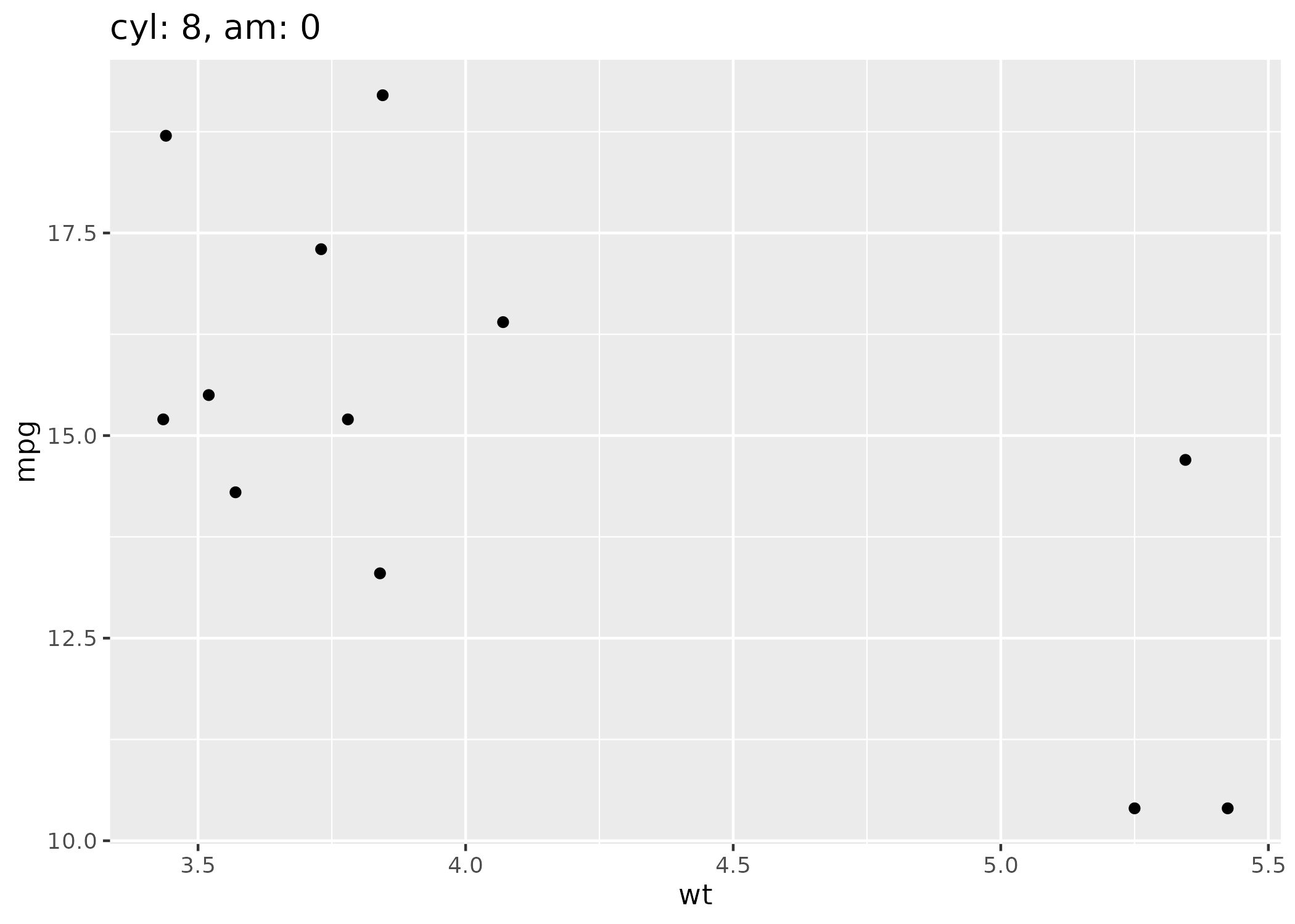
Simply format the path to the saved figure like  and execute render_tabset() as before.
# directory for saving figuresdir_fig <-"figures"# create the directorydir.create(dir_fig)# new sample datadf3 <- df2 |>mutate(# Create file names to savefig_path =file.path( dir_fig,paste0(gsub("[[:punct:]]\\s", "_", title), "_map2_chr.png") ),# To make the return value a character vector, use `map2_chr()`fig_path_md =map2_chr( fig, fig_path, \(p, path) {# save figureggsave(path, p)# format path to markdown stylesprintf("", path, path) } ) ) |>select(cyl, am, fig_path_md)df3
# A tibble: 6 × 3
cyl am fig_path_md
<chr> <chr> <chr>
1 cyl: 6 am: 1  + map() method with row-wise data.
df3_rowwise <- df2_rowwise |>mutate(# Create file names to savefig_path =file.path( dir_fig,paste0(gsub("[[:punct:]]\\s", "_", title), "_rowwise.png") ),fig_path_md = {# save figureggsave(fig_path, fig)# format path to markdown stylesprintf("", fig_path, fig_path) } ) |>select(cyl, am, fig_path_md)df3_rowwise
# A tibble: 6 × 3
# Rowwise: cyl, am
cyl am fig_path_md
<chr> <chr> <chr>
1 cyl: 4 am: 0 , it seems JavaScript dependencies need to be resolved. The easiest way seems to output them once in a separate chunk.
For example, we use {plotly} to create interactive figures. Simply apply plotly::ggplotly() to the already created ggplot object. Then it needs to be passed to htmltools::div().
Here we will show you how to use render_tabset() in a popular package for rendering tables. This example uses knitr::kable(), gt::gt(), gt::opt_interactive(), flextable::flextable(), DT::datatable(), reactable::reactable() and tinytable::tt().
tables <- df2 |>select(cyl, am, data) |>mutate(kable =map(data, knitr::kable),gt =map(data, gt::gt),gt_interactive =map(gt, gt::opt_interactive),tt =map(data, tinytable::tt),flex =map_chr( data, \(data) { flextable::flextable(data) |> knitr::knit_print() } ),DT =map( data, \(data) { DT::datatable(data) |> htmltools::div() } ),reac =map( data, \(data) { reactable::reactable(data) |> htmltools::div() } ),section_kable ="#### knitr::kable()",section_gt ="#### gt::gt()",section_gt_interactive =paste("#### gt::gt() |> gt::opt_interactive()","(and run in a separate chunk)" ),section_tt ="#### tinytable::tt()",section_flex =paste("#### flextable::flextable() |> knitr::knit_print()","(using map_chr())" ),section_DT =paste("#### DT::datatable() |> htmltools::div()","(and run in a separate chunk)" ),section_reac =paste("#### reactable::reactable() |> htmltools::div()","(and run in a separate chunk)" ) )tables
knitr::kable(), gt::gt(), and tinytable::tt() are the simplest.
The output of flextable::flextable() is managed by the method knitr::knit_print(). After execution, raw HTML is obtained, which is turned into a character type column using map_chr().
gt::opt_interactive(), {DT} and {reactable} use JavaScript. They should be wrapped with htmltools::div(), except for gt::opt_interactive(), and run in a separate chunk to resolve javascript dependencies. Don’t forget #| include: false.
```{r}#| include: false# Here mtcars are specified as dummy data, # but any data frame should be acceptablegt::gt(mtcars) |> gt::opt_interactive()DT::datatable(mtcars)reactable::reactable(mtcars)```
Then execute render_tabset(). To make the results easier to see, sections are also to be added.
DT::datatable() |> htmltools::div() (and run in a separate chunk)
reactable::reactable() |> htmltools::div() (and run in a separate chunk)
References
As this function is focused on quickly and dynamically generating tabsets and chunks, it is difficult to customize it on a chunk-by-chunk basis. The regular way to dynamically create chunks is to use functions such as knitr::knit(), knitr::knit_child(), knitr::knit_expand(), etc. For more information on these, see the following links.
Heiss, Andrew. 2024. “Guide to Generating and Rendering Computational Markdown Content Programmatically with Quarto.” November 4, 2024. https://doi.org/10.59350/pa44j-cc302
# save the session info as an objectsess <- sessioninfo::session_info(pkgs ="attached")# inject the Quarto infosess$platform$quarto <-paste( quarto::quarto_version(),"@",normalizePath(quarto::quarto_path()))# print it outsess
---title: "Get started"format: html: code-link: true code-tools: true toc: true toc-location: right toc-expand: truedate: last-modifiedknitr: opts_chunk: message: false eval: true---## Introduction[Tabset](https://quarto.org/docs/output-formats/html-basics.html#tabsets) is an interactive panel in Quarto html documents.::: {.panel-tabset}## ATab content for A## BTab content for B:::This was written as follows.```` markdown::: {.panel-tabset}## ATab content for A## BTab content for B:::````It is troublesome to rewrite manually in the following cases: - There are many tabs. - The number of tabs increases or decreases. - You want to write nested tabs. The `quartabs::render_tabset()` takes a data frame as input and outputs it dynamically.**Note that the chunk option must be `results: asis`**.```{r}#| results: asis#| echo: fenceddata.frame(tab =c("A", "B"),value =c("Tab content for A", "Tab content for B")) |> quartabs::render_tabset(tab, value)```## Basic usageHere are basic examples. First, load the libraries used in this demo and create sample data.```{r}#| message: falselibrary(quartabs)library(tibble)library(dplyr)library(purrr)library(tidyr)library(plotly)library(htmltools)library(knitr)library(gt)library(DT)library(tinytable)library(reactable)library(flextable)# sample datadf1 <-tibble(# id: intentionally created in descending order for the examples shown laterid =paste0("id", 6:1),group1 =c(rep("A", 3), rep("B", 3)),group2 =rep(c("X", "Y", "Z"), 2),var1 =1:6,var2 =list(1, 2, 3, 4, 5, 6),var3 =factor(letters[1:6]))df1```### `tabset_vars`, `output_vars`The `tabset_vars` argument specifies columns to display as tab labels. The `output_vars` argument specifies the columns to display in the tab.::: {.callout-note icon="true"}## Don't forget!Make sure to set the chunk option to `results: asis`.Default chunk options can be changed if necessary.```` rknitr::opts_chunk$set(results ="asis")````:::```{r}#| results: asis#| echo: fenceddf1 |>render_tabset(tabset_vars = id,output_vars = var1 )```The data is sorted internally by `tabsest_vars`. Therefore, the tabsets were displayed in ascending order.Multiple `tabset_vars` and `output_vars` are acceptable. For multiple `tabset_vars`, they are displayed nested.```{r}#| results: asis#| echo: fenceddf1 |>render_tabset(c(group1, group2), c(var1, var2, var3))```:::{.callout-tip}## `cat()` or `print()``cat()` is used internally for non-list columns to avoid unnecessary prefixes such as "[1]" in the output. On the other hand, `print()` is used for list columns.For example, `var1` displays "1", while `var2` of type list displays "[1] 1".:::### Factor, Date and POSIXt displaysIn `render_tabset()`, `cat()` is used to output for columns that are not list types.However, if `cat()` is used, factor, Date, POSIXt are output as an integer. So, if these are included in `tabset_vars` or `output_vars`, it is converted internally to string (after sorting by `tabset_vars`).Here are some simple examples. First, define test objects.```{r}(test_factor <-factor("a"))(test_date <-as.Date("2025-01-01"))(test_posixct <-as.POSIXct("2025-01-01 12:34:56", tz ="UTC"))```Using `cat()` results in output as a number. This is not usually the expected output.```{r}cat(test_factor)cat(test_date)cat(test_posixct)```Therefore, `render_tabset()` uses `cat()` after converting it internally to a string as follows.```{r}cat(as.character(test_factor))cat(as.character(test_date))cat(as.character(test_posixct))```### `layout`How can I display the content in a tabset horizontally?In Quarto, `layout-ncol` can be used.```{r}#| results: asis#| layout-ncol: 3#| echo: fenceddf1 |>render_tabset(c(group1, group2), c(var1, var2, var3))```Oops, the entire tabset is now a third of the width.We want the content within to be displayed side by side without changing the width of the tabset.This is where the `layout` argument comes in handy.```{r}#| results: asis#| echo: fenceddf1 |>render_tabset(c(group1, group2),c(var1, var2, var3),layout ="::: {layout-ncol=3}" )```In fact, the above `layout` is a shortcut to something like this:```{r}#| results: asis#| echo: fenceddf1 |>mutate(layout_start ="::: {layout-ncol=3}",layout_end =":::" ) |>render_tabset(c(group1, group2),c(layout_start, var1, var2, var3, layout_end) )```For more information about `layout`, see [Custom Layouts](https://quarto.org/docs/authoring/figures.html#complex-layouts). :::{.callout-warning}* In narrower displays, such as on smartphones, the layout may not appear to work.* The `layout` argument is intended for very simple use cases, so complex layouts may not work.:::### `heading_levels`Use the `heading_levels` argument if you want the heading to be displayed as normal headings instead of tabsets. `heading_levels` and `tabset_vars` correspond in order.Each `tabset_vars` is expressed as the heading of specified in `heading_levels`.If the element of `heading_levels` is `NA`, then the element of its `tabset_vars` is represented as tabset.#### Example 1 For example, `group1` should be tabset and `group2` should be h4 heading.```{r}#| results: asis#| echo: fenceddf1 |>render_tabset(c(group1, group2),c(var1, var2, var3),heading_levels =c(NA, 4) )```#### Example 2Conversely, `group1` should be heading 4 and `group2` should be tabset.```{r}#| results: asis#| echo: fenceddf1 |>render_tabset(c(group1, group2),c(var1, var2, var3),heading_levels =c(4, NA) )```#### Example 3Set `group1` to heading 4 and `group2` to heading 5 (no tabset).```{r}#| results: asisdf1 |>render_tabset(c(group1, group2),c(var1, var2, var3),heading_levels =c(4, 5) )```### `pills`As of 2025-03-05, the latest version of Quarto is 1.6, but the Bootstrap version used appears to be Bootstrap 5.2.2, which was [introduced with Quarto 1.4](https://quarto.org/docs/download/changelog/1.4/#:~:text=for%20HTML%20output-,(%235210)%3A%20Update%20to%20Bootstrap%205.2.2,-(%235393)%3A%20Properly).Several tab customisations are available in Bootstrap 5.2. One of these is [pills](https://getbootstrap.com/docs/5.2/components/navs-tabs/#pills).```{r}#| results: asis#| echo: fenceddf1 |>render_tabset(c(group1, group2),c(var1, var2, var3),pills =TRUE )```### `tabset_width`Similarly, you can choose from three [fill and justify](https://getbootstrap.com/docs/5.2/components/navs-tabs/#fill-and-justify). In the following, long labels are created for the sake of example and displayed at half width.**"default"**```{r}#| results: asis#| layout-ncol: 2#| echo: fenceddf1_long_label <- df1 |>mutate(group1 =paste("This is a long label for", group1) )df1_long_label |>render_tabset(c(group1, group2),c(var1, var2, var3),tabset_width ="default" )```**"fill"**```{r}#| results: asis#| layout-ncol: 2#| echo: fenceddf1_long_label |>render_tabset(c(group1, group2),c(var1, var2, var3),tabset_width ="fill" )```**"justified"**```{r}#| results: asis#| layout-ncol: 2#| echo: fenceddf1_long_label |>render_tabset(c(group1, group2),c(var1, var2, var3),tabset_width ="justified" )```## Figures and tablesThis section shows more practical examples.Use the `mtcars` dataset, grouped by `cyl` and `am`, to create figures and tables showing the relationship between `wt` and `mpg`.`render_tabset()` was originally created to represent figures and tables as tabsets, with nested data frames as input.Nesting approach is useful when the same operation is performed on each group.### `nest() + map()`We shows how to use `tidyr::nest()` and `purrr::map()` combination.For more information on the nest, see follows:- [Nested data](https://tidyr.tidyverse.org/articles/nest.html)- [23 Model basics](https://r4ds.had.co.nz/model-basics.html)**Japanese**- [TokyoR #108 Nested Data Handling](https://speakerdeck.com/kilometer/tokyor-number-108-nesteddatahandling)- [nested data で ggplot](https://qiita.com/kilometer/items/7f99c0a9af6d7ce43485)```{r}# new sample datadf2 <- mtcars |># make groups more explicitmutate(cyl =paste("cyl:", cyl),am =paste("am:", am) ) |># nestnest(.by =c(cyl, am)) |>mutate(# create titles for figurestitle =paste(cyl, am, sep =", "),# create scatter plotsfig =map2( data, title, \(data, title) { data |>ggplot(aes(wt, mpg)) +geom_point() +labs(title = title) } ),# create tablestbl =map( data, \(data) { data |>select(wt, mpg) |> knitr::kable() } ) )df2```Figures and tables have been created for the `fig` and `tbl` columns respectively.### `nest_by() + list()`Another method is to use `dplyr::nest_by()` and `list()`. This approach is simpler and more intuitive to write.For more information, see follows:- [Row-wise operations](https://dplyr.tidyverse.org/articles/rowwise.html)```{r}df2_rowwise <- mtcars |># make groups more explicitmutate(cyl =paste("cyl:", cyl),am =paste("am:", am) ) |># nestnest_by(cyl, am) |>mutate(# create titles for figurestitle =paste(cyl, am, sep =", "),# create scatter plotsfig =list( data |>ggplot(aes(wt, mpg)) +geom_point() +labs(title = title) ),# create tablestbl =list( data |>select(wt, mpg) |> knitr::kable() ) )df2_rowwise```This way, the values of other columns in the `list()` can be used freely. (In the `nest() + map()` method, it was necessary to define in advance which columns to use when calling in the `map()`).The outputs are grouped row-wise and already sorted by `cly` and `am`.### FiguresIn the following, `df2` is used. (Works in the same way if you use `df2_rowwise`).::: {.callout-warning}When specifying a list-type column that includes ggplot objects in `output_vars`, setting the chunk option `echo: fenced` may cause the plots to not display correctly.:::```{r}#| results: asisdf2 |> render_tabset(c(cyl, am), fig)``````{r}#| results: asis#| echo: falsedf2 |>render_tabset(c(cyl, am), fig)```### Tables```{r}#| results: asis#| echo: fenceddf2 |>render_tabset(c(cyl, am), tbl)```### Figures and tables```{r}#| results: asisdf2 |> render_tabset(c(cyl, am), c(fig, tbl))``````{r}#| results: asis#| echo: falsedf2 |>render_tabset(c(cyl, am), c(fig, tbl))```### layoutUse the `layout` argument to display figure and table side by side with a width of 7:3.```{r}#| results: asisdf2 |> render_tabset( c(cyl, am), c(fig, tbl), layout = '::: {layout="[7, 3]"}' )``````{r}#| results: asis#| echo: falsedf2 |>render_tabset(c(cyl, am),c(fig, tbl),layout ='::: {layout="[7, 3]"}' )```## Advanced examples### Pre-saved figuresSimply format the path to the saved figure like `` and execute `render_tabset()` as before.```{r}#| include: false#| echo: false# This is code to clean up the gh-pages branch.# So this is intentionally hidden.# directory for saving figuresdir_fig <-"figures"# delete the directory if it existsif (dir.exists(dir_fig)) {unlink(dir_fig, recursive =TRUE)}``````{r}# directory for saving figuresdir_fig <-"figures"# create the directorydir.create(dir_fig)# new sample datadf3 <- df2 |>mutate(# Create file names to savefig_path =file.path( dir_fig,paste0(gsub("[[:punct:]]\\s", "_", title), "_map2_chr.png") ),# To make the return value a character vector, use `map2_chr()`fig_path_md =map2_chr( fig, fig_path, \(p, path) {# save figureggsave(path, p)# format path to markdown stylesprintf("", path, path) } ) ) |>select(cyl, am, fig_path_md)df3```Then execute `render_tabset()` as in basic usage.```{r}#| results: asis#| echo: fenceddf3 |>render_tabset(c(cyl, am), fig_path_md)```:::{.callout-tip}## Using row-wise dataReplace the above `nest() + map()` method with row-wise data.```{r}df3_rowwise <- df2_rowwise |>mutate(# Create file names to savefig_path =file.path( dir_fig,paste0(gsub("[[:punct:]]\\s", "_", title), "_rowwise.png") ),fig_path_md = {# save figureggsave(fig_path, fig)# format path to markdown stylesprintf("", fig_path, fig_path) } ) |>select(cyl, am, fig_path_md)df3_rowwise```Then execute `render_tabset()` as in basic usage.```{r}#| results: asis#| echo: fenceddf3_rowwise |>render_tabset(c(cyl, am), fig_path_md)```:::### Resolve JavaScript dependenciesWhen outputting tables or figures that use JavaScript (such as `{plotly}`, `{leaflet}`, `{DT}`, `{reactable}`, etc.), it seems JavaScript dependencies need to be resolved. The easiest way seems to output them once in a separate chunk.References:- [offline plots in for loops - github](https://github.com/plotly/plotly.R/issues/273)- [Using ggplotly and DT from a for loop in Rmarkdown - stackoverflow](https://stackoverflow.com/questions/60685631/using-ggplotly-and-dt-from-a-for-loop-in-rmarkdown/62599342#62599342)- [plotly objects are invisible in R Markdown - stackoverflow](https://stackoverflow.com/questions/75992729/plotly-objects-are-invisible-in-r-markdown)For example, we use `{plotly}` to create interactive figures. Simply apply `plotly::ggplotly()` to the already created ggplot object. **Then it needs to be passed to `htmltools::div()`**.```{r}df4 <- df2 |>mutate(fig_plotly =map( fig, \(p) {ggplotly(p) |> htmltools::div() } ) ) |>select(cyl, am, fig_plotly)df4```As mentioned above, we need a chunk that only runs `plot_ly()`. Set `#| include: false` so that this chunk and its output will not appear on the report.```{r}#| include: falseplot_ly()``````{r}#| include: falseplot_ly()```Then execute `render_tabset()` as in basic usage.```{r}#| results: asis#| echo: fenceddf4 |>render_tabset(c(cyl, am), fig_plotly)```### TablesHere we will show you how to use `render_tabset()` in a popular package for rendering tables.This example uses `knitr::kable()`, `gt::gt()`, `gt::opt_interactive()`, `flextable::flextable()`, `DT::datatable()`, `reactable::reactable()` and `tinytable::tt()`.```{r}tables <- df2 |>select(cyl, am, data) |>mutate(kable =map(data, knitr::kable),gt =map(data, gt::gt),gt_interactive =map(gt, gt::opt_interactive),tt =map(data, tinytable::tt),flex =map_chr( data, \(data) { flextable::flextable(data) |> knitr::knit_print() } ),DT =map( data, \(data) { DT::datatable(data) |> htmltools::div() } ),reac =map( data, \(data) { reactable::reactable(data) |> htmltools::div() } ),section_kable ="#### knitr::kable()",section_gt ="#### gt::gt()",section_gt_interactive =paste("#### gt::gt() |> gt::opt_interactive()","(and run in a separate chunk)" ),section_tt ="#### tinytable::tt()",section_flex =paste("#### flextable::flextable() |> knitr::knit_print()","(using map_chr())" ),section_DT =paste("#### DT::datatable() |> htmltools::div()","(and run in a separate chunk)" ),section_reac =paste("#### reactable::reactable() |> htmltools::div()","(and run in a separate chunk)" ) )tables````knitr::kable()`, `gt::gt()`, and `tinytable::tt()` are the simplest.The output of `flextable::flextable()` is managed by the method `knitr::knit_print()`. After execution, raw HTML is obtained, which is turned into a character type column using `map_chr()`.`gt::opt_interactive()`, `{DT}` and `{reactable}` use JavaScript. They should be wrapped with `htmltools::div()`, except for `gt::opt_interactive()`, and run in a separate chunk to resolve javascript dependencies. Don't forget `#| include: false`.```{r}#| include: false# Here mtcars are specified as dummy data, # but any data frame should be acceptablegt::gt(mtcars) |> gt::opt_interactive()DT::datatable(mtcars)reactable::reactable(mtcars)``````{r}#| include: falsegt::gt(mtcars) |> gt::opt_interactive()DT::datatable(mtcars)reactable::reactable(mtcars)```Then execute `render_tabset()`. To make the results easier to see, sections are also to be added.```{r}#| results: asis#| echo: fencedtables |>render_tabset(c(cyl, am),c( section_kable, kable, section_gt, gt, section_gt_interactive, gt_interactive, section_tt, tt, section_flex, flex, section_DT, DT, section_reac, reac ) )```## ReferencesAs this function is focused on quickly and dynamically generating tabsetsand chunks, it is difficult to customize it on a chunk-by-chunk basis.The regular way to dynamically create chunks is to use functions such as`knitr::knit()`, `knitr::knit_child()`, `knitr::knit_expand()`, etc.For more information on these, see the following links.- Heiss, Andrew. 2024. “Guide to Generating and Rendering Computational Markdown Content Programmatically with Quarto.” November 4, 2024.<https://doi.org/10.59350/pa44j-cc302>- <https://bookdown.org/yihui/rmarkdown-cookbook/child-document.html#child-document>- <https://bookdown.org/yihui/rmarkdown-cookbook/knit-expand.html>## Session Info```{r}#| warning: false# save the session info as an objectsess <- sessioninfo::session_info(pkgs ="attached")# inject the Quarto infosess$platform$quarto <-paste( quarto::quarto_version(),"@",normalizePath(quarto::quarto_path()))# print it outsess```